Forget Determinism, see Randomness in Action: How to Model Stock Price

Our intuition can be easily twisted with a simple thought experiment. If someone offers you a million dollars at once or gives you a penny that doubles every day for a month, what would you choose? The choice is yours, but I would suggest choosing the penny.

What is important in the previous puzzle is that our doubling penny follows a geometric progression law. It is the law of expressing changes in terms of previous states in a multiplicative manner. This is why it easily breaks our intuition on how rapidly some measurable quantity can escalate in a positive or negative direction.

This vigorously exploding tendency depending on the previous states is essential for modeling some random processes. In the previous blog posts, we introduced the Random Walk, and out of it, we constructed the Standard Brownian Motion and the Brownian Motion with drift and volatility. However, these processes exhibit an additive behavior without explicitly embedding the rate of change with respect to the previous time steps.

In this blog, we dig more and introduce the Geometric Brownian Motion. It handles products of independent increments rather than a sum of independent increments. This multiplicative nature amplifies the rate of relative changes in short-time intervals, which in turn makes the process well suited for a plethora of applications. For instance, one of the most common applications is to model stock prices or even whole stock exchange indices.

In the same fashion as before, we use Python's numerical packages to implement the Geometric Brownian Motion. Additionally, we analyze and simulate some fascinating properties of this process using Matplotlib's Animation API. Stay tuned!

The Natural Language of Growth

Random Walks follow an additive law, which means every succeeding value is the sum of the preceding one and a random increment (positive or negative), i.e.

The quantity we add to the preceding value defines the rate of change of the process. In this case, the rate is not directly related to the previous value, thus posing a major limitation.

A more intuitive way is to express the rate of change in relative terms to the previous values. For instance, think about the interest rate, a well-defined quantity in the banking sector. It is always expressed as a percentage of the principal, i.e. the initial value.

For demonstration purposes, let's take two very simple processes in the discrete space, one multiplicative and another additive as defined below:

The rate of change is defined as the speed at which one variable changes in a short amount of time. In our example, for the two discrete-time processes, the rate of change is illustrated below:

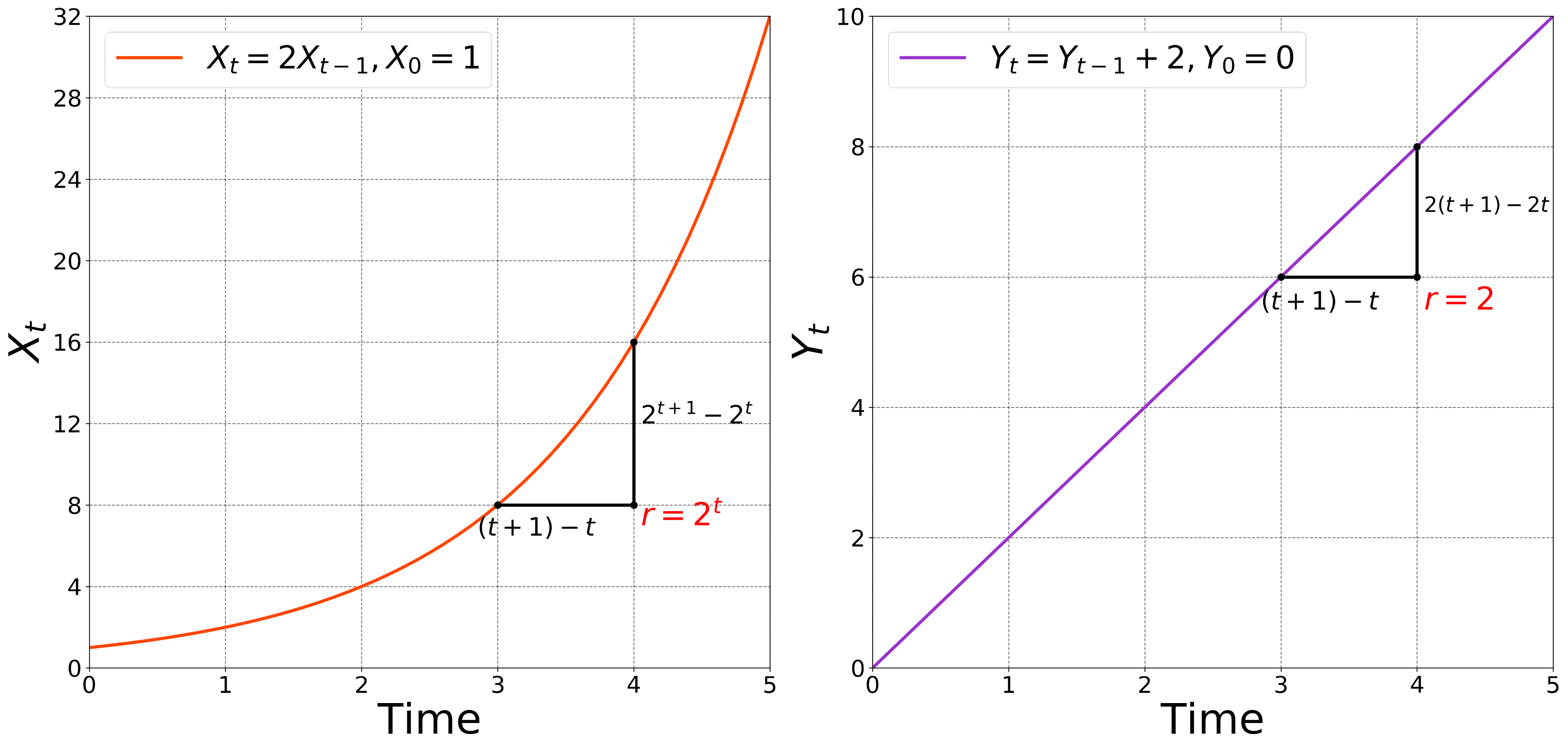
Fig. 1: Rate of change between additive and multiplicative increments

On one hand, the rate of change for the multiplicative process depends directly on the previous value. On the other hand, the rate of change for the additive process is constant without any relation to the process itself. This is quite constraining because we do not have an anchor to refer to.

In order to transform a process with additive increments, like the Random Walk to a process with multiplicative increments, we use a simple trick. Power with a sum in the exponent becomes a product of powers, as shown below:

Most frequently in math, we use the number \( e \) as a base of power, since it represents the natural language of growth. It simplifies the operations and removes all hurdles in the process of derivation and integration. This leads us to the definition of a Geometric Brownian Motion.

Definition of Geometric Brownian Motion

The Geometric Brownian Motion is a simple transformation of the Drifted Brownian Motion, yet so essential. We transform a process that can handle the sum of independent normal increments to a process that can handle the product of independent increments, as defined below:

This process follows a log-normal distribution, which implies that the generated values never go below zero. This comes quite handy for modeling stock prices and stock exchange indices because they share the same characteristic, they are never negative.

Our Python implementation is based on our previous work on Standard Brownian Motion. By reusing that module, the Geometric Brownian Motion is implemented as follows:

 1
 2
 3
 4
 5
 6
 7
 8
 9
10
11
12
13
14
15
16
17
18
19
20
21
22
23

def geometric_brownian_motion(G0, mu, sigma, N, T):
    """Simulates a Geometric Brownian Motion.

    :param float G0: initial value
    :param float mu: drift coefficient
    :param float sigma: diffusion coefficient
    :param int N: number of discrete steps
    :param int T: number of continuous time steps
    :return list: the geometric Brownian Motion
    """
    # the normalizing constant
    dt = 1. * T/N
    # standard brownian motion
    W, _ = brownian_motion(N, T ,1.0)
    # generate the time steps
    time_steps = np.linspace(0.0, N*dt, N+1)

    # calculate the geometric brownian motion
    G = G0 * np.exp(mu * time_steps + sigma * W)
    # replace the initial value
    G[0] = G0

    return G

This process has some very interesting properties to analyze, related to its mean and variance. We cover this in the following section.

Zero Mean, Infinite Variance

The random processes have mean and variance as a function of the time, which makes them interesting for analysis. Without going into the details of their derivation, the mean and variance of the Geometric Brownian Motion are given below:

The major limitation of these metrics is their determinism. A more realistic scenario would be to model them in a stochastic manner as well. The Python implementation is quite straightforward as shown in the code snippet below:

 1
 2
 3
 4
 5
 6
 7
 8
 9
10
11
12
13
14
15
16
17
18
19
20
21
22
23
24
25
26
27
28
29
30
31
32

import numpy as np
def gbm_mean(G0, mu, sigma, N, T):
    """Simulates the mean of the Geometric Brownian Motion, which is:
        E(t) = G0*e^{(mu + sigma^{2}/2)*t}
    :param float G0: initial value
    :param float mu: drift coefficient
    :param float sigma: diffusion coefficient
    :param int N: number of discrete steps
    :param int T: number of continuous time steps
    """
    # generate the time steps
    t = np.linspace(0.0, T, N+1)
    # calculate the mean
    E = G0 * np.exp((mu + 0.5*sigma**2)*t)

    return E

def gbm_var(G0, mu, sigma, N, T):
    """Simulates the variance of the Geometric Brownian Motion, which is:
        Var(t) = G0^2 * e^{(2*mu + sigma^{2})*t} * (e^{sigma^{2}*t} - 1)
    :param float G0: initial value
    :param float mu: drift coefficient
    :param float sigma: diffusion coefficient
    :param int N: number of discrete steps
    :param int T: number of continuous time steps
    """
    # generate the time steps
    t = np.linspace(0.0, T, N+1)
    # calculate the variance
    V = G0**2 * np.exp(t * (2*mu + sigma**2)) * (np.exp(t * sigma**2) - 1)

    return V

As we can see the drift and volatility coefficients define the nature of the mean and variance, which means they have an important role. The interplay between them can shape the mean and variance in many different and interesting scenarios. One particular and fascinating property is that we can have zero mean and infinite variance. Although it seems bizarre, we observe this phenomenon as soon as the following condition holds:

We make an animated visualization using the Matplotlib's Animation API to get more sense on this and go from "I think I understand" to "I fully understand". This facilitates the process of grasping and understanding the concepts in an enticing manner, as depicted below:

Animation: Zero Mean and Infinite Variance

Now we conclude that what we observed is coherent with the short mathematical analysis we made. The mean indeed decays to zero, while the variance explodes to infinity.

The full source code related to all we have discussed during this blog can be found on GitHub. For more information, please follow me on Twitter.

If you liked what you just saw, it would be really helpful to subscribe to the mailing list below. You will not get spammed that's a promise! You will get updates for the newest blog posts and visualizations from time to time.

Key takeaways

During this blog, we learned about the Geometric Brownian Motion, which is well suited for expressing the rate of change in multiplicative terms. It handles products of random increments, thus following a log-normal distribution. Therefore, the generated values are more easily expressed in relative terms of the previous ones and they are never negative. This makes the process a good match to model stock prices and stock exchange indices.

On top of everything, this process is the foundation of the Stochastic Differential Equations and Stochastic Integration, which we will start covering in the next few blogs.

Appendix

In our visualization above, we only saw one single realization of the Geometric Brownian Motion. However, the process can yield any number of hypothetical paths, depending on the initial conditions. To visualize this pure uncertainty of the process, we generate 10 processes with exactly the same parameters, only different initial seed. The result is visualized in the animation below:

Animation: Same parameters, different seeds

References

[1] Peter Olofsson, Mikael Andersson, "Probability, Statistics, and Stochastic Processes"