Simple but Stunning: Animated Cellular Automata in Python

The automation epitomizes the last few decades of rapid technological development where many processes take place without human intervention. But what exactly does it mean?

Automaton (noun):

• : a mechanism that is relatively self-operating
• : a machine or control mechanism designed to follow a predetermined sequence of operations

These are the two most common definitions of the word automaton, related to the word automation, automatic or automatically.

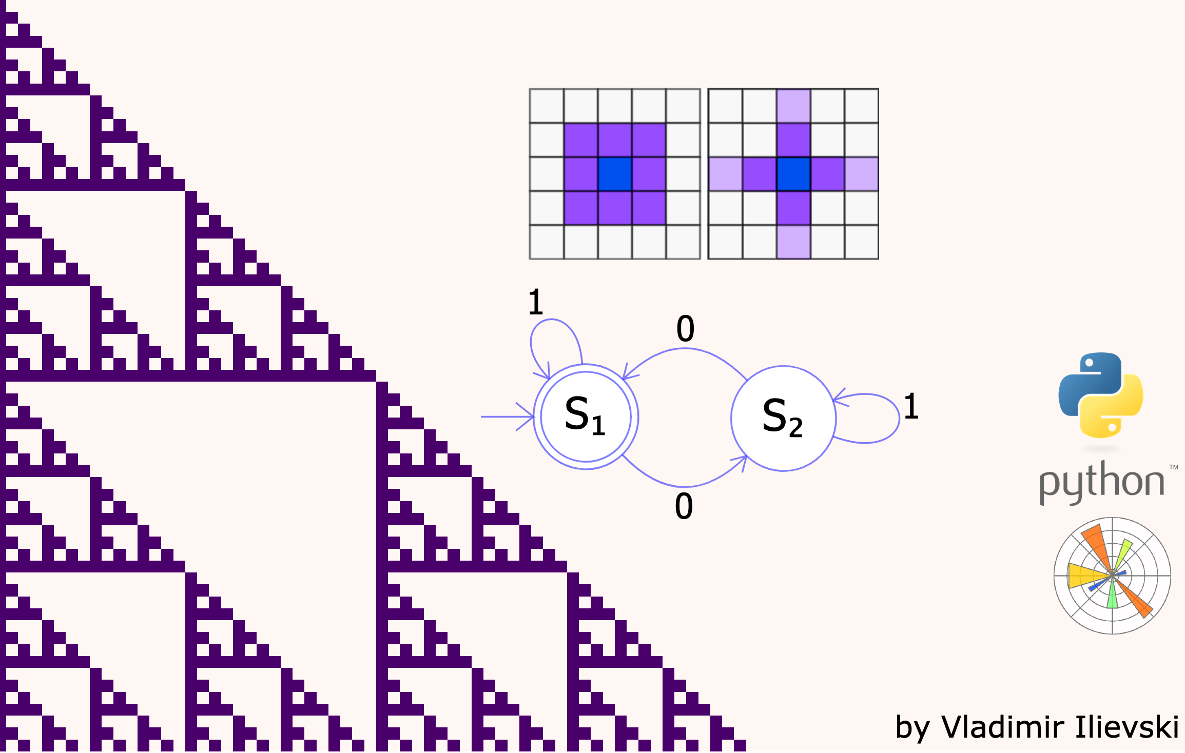
In the very same sense, as you might already know, one automaton is always in some precise and unequivocal state. It transitions to another precisely defined state given some instruction. We can visually represent any automata using a directed graph, where states are represented with nodes, while the transitions with edges. One very simple automaton is shown in the figure below:

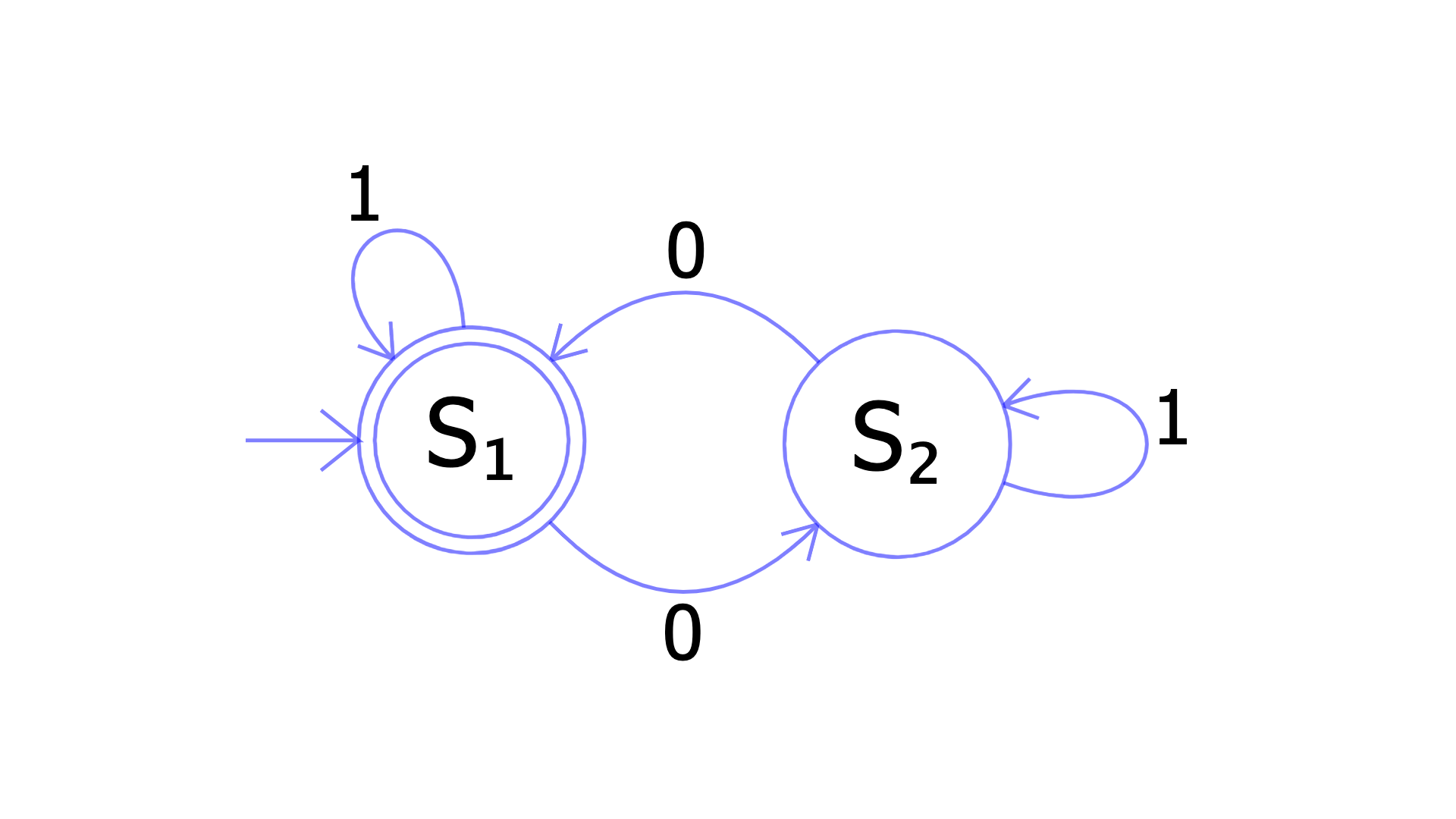
Fig. 1: Simple Automaton with two states. Taken from Wikipedia.

This is the fundamental principle of the entire computing machinery we use today. Starting from the very simple coffee machine at your home up to the very complex device on which you read this story. All these machines follow a set of instructions and transition from one state to another.

Contrary to this deterministic definition of automata, what happens if we have some arbitrary program? What if we have a program that does not rely on receiving some precise set of instructions, but rather arbitrary ones depending on its current state. Something more closely related to the evolution of the living organisms in nature.

I am not intending to reinvent the wheel here, many scientists had the same questions a long time ago. It is only to give the intuition and motivation behind the conception and definition of the cellular automata.

The cellular automaton relies on and is motivated by the principles of the living organisms in nature. It consists of a grid of cells each having some state. Every cell advances in time according to some mathematical function of the neighboring cells. Thus, the entire automata behave like a living organism.

By the end of this blog post, you will be able to understand and see the potential of cellular automata. First, we'll delve into the formal definition and elaborate more on some particular cases. Then to complete the puzzle, we will see how to implement some interesting cellular automata in Python complemented with interesting animated visualizations using Matplotlib. Stay tuned!

Definition of Cellular Automaton

A cellular automaton is fully defined by three key elements:

1. Collection of “colored” cells each having a state;
2. The cells are distributed on a grid with a predefined shape and
3. The cells update their state according to a rule-based on the neighboring cells.

For instance, we can take the most simple case when the state of the cell is either on or off, or in other words either 1 or 0.

The grid in general is represented as a rectangle with a shape of \( M \times N \), meaning it has M rows and N columns. Then, each cell is represented as a small rectangle on the grid.

Knowing all of this, we can define what cells are considered neighbors of a given cell. For a squared grid, the two most common neighborhoods are:

1. Moore neighborhood (squared neighborhood) as shown on the left of Fig. 2;
2. von Neumann neighborhood (diamond-shaped) as shown on the right of Fig. 2.

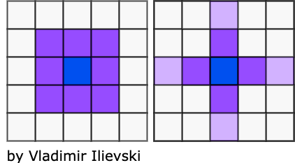
Fig. 2: Moore vs Von Neumann neighborhoods

Now, the update rule is simply a function of the current cell state and the states of the cells in its pre-defined neighborhood. The only missing piece of the puzzle is the initial state of the automaton, which might be deterministic or random.

The initial condition, the 2-dimensional grid, the type of neighborhood, and the update rule give rise to infinitely many scenarios that are difficult to analyze. For this reason, we’ll focus only on the most simple case of cellular automata, namely the elementary cellular automata.

Elementary Cellular Automata

The elementary cellular automata are the simplest non-trivial automata. They are one-dimensional, meaning there is only one row of cells. Each cell is having two possible states (0 or 1), and its neighbors are the adjacent cells on either side of it as shown in the figure below:

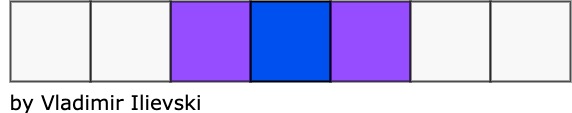
Fig. 3: Elementary cellular automaton

Every cell with its two neighboring cells forms a patch of 3 cells, each of which can have 2 states: either 0 or 1. Plugging a simple variation with repetition gives us \( 2^{3} = 8 \) possible options: 000, 001, 010, 011, 100, 101, 110, 111 (the numbers from 0 to 7 in binary format).

Using these 8 options, we can decide whether the next state of the central cell will take a value of 0 or 1. This is equivalent to asking the question: in how many possible ways one can arrange 8 bits? Same as before, this gives us \( 2^{8} = 256 \) options for an update rule. Following the same analogy, these are the numbers from 0 to 255 in binary format. For this reason, the rules are referred to by their ordering number.

For example, since \( 150_{2} = 10010110 \), the update rule number 150 is illustrated in the figure below:

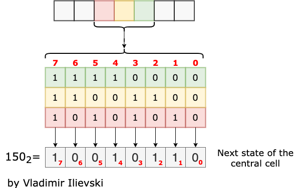
Fig. 4: Update rule 150

Next, we’ll see how to turn this into a Python implementation and a visualization using Matplotlib.

Python Implementation

The first thing to implement is the update rule. Given the state of each cell in the row at some time step T (denoted as x) and the update rule number, we need to derive the state of each cell in the next time step. To do so, we use the following code:

 1
 2
 3
 4
 5
 6
 7
 8
 9
10
11
12
13
14
15
16
17
18
19
20

import numpy as np

powers_of_two = np.array([[4], [2], [1]])  # shape (3, 1)

def step(x, rule_binary):
    """Makes one step in the cellular automaton.

    Args:
        x (np.array): current state of the automaton
        rule_binary (np.array): the update rule

    Returns:
        np.array: updated state of the automaton
    """
    x_shift_right = np.roll(x, 1)  # circular shift to right
    x_shift_left = np.roll(x, -1)  # circular shift to left
    y = np.vstack((x_shift_right, x, x_shift_left)).astype(np.int8)  # stack row-wise, shape (3, cols)
    z = np.sum(powers_of_two * y, axis=0).astype(np.int8)  # LCR pattern as number

    return rule_binary[7 - z]

First, we shift the state of each cell to the right, then to the left in a circular fashion. Next, we stack one upon the other the left shift, the current and the right shift of the cells’ states. This gives us a structure where each column has three elements with a value of either 0 or 1. It means that one column represents one number from 0 to 7 in a binary format. We use this value as an index in the update rule which determines the next state of the central cell. The entire procedure is sketched in the figure below:

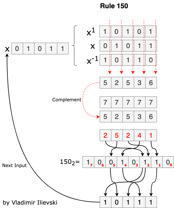
Fig. 5: Explanation of the function step

Having the update rule implemented, the rest of the implementation is quite straightforward. We have to initialize the cellular automaton and then run it for a pre-defined number of time steps. The Python implementation is given below:

 1
 2
 3
 4
 5
 6
 7
 8
 9
10
11
12
13
14
15
16
17
18
19
20
21
22
23
24
25
26
27
28
29
30
31
32
33
34
35
36
37
38
39
40
41
42
43

import numpy as np

def cellular_automaton(rule_number, size, steps,
                       init_cond='random', impulse_pos='center'):
    """Generate the state of an elementary cellular automaton after a pre-determined
    number of steps starting from some random state.

    Args:
        rule_number (int): the number of the update rule to use
        size (int): number of cells in the row
        steps (int): number of steps to evolve the automaton
        init_cond (str): either `random` or `impulse`. If `random` every cell
        in the row is activated with prob. 0.5. If `impulse` only one cell
        is activated.
        impulse_pos (str): if `init_cond` is `impulse`, activate the
        left-most, central or right-most cell.

    Returns:
        np.array: the final state of the automaton
    """
    assert 0 <= rule_number <= 255
    assert init_cond in ['random', 'impulse']
    assert impulse_pos in ['left', 'center', 'right']

    rule_binary_str = np.binary_repr(rule_number, width=8)
    rule_binary = np.array([int(ch) for ch in rule_binary_str], dtype=np.int8)
    x = np.zeros((steps, size), dtype=np.int8)

    if init_cond == 'random':  # random init of the first step
        x[0, :] = np.array(np.random.rand(size) < 0.5, dtype=np.int8)

    if init_cond == 'impulse':  # starting with an initial impulse
        if impulse_pos == 'left':
            x[0, 0] = 1
        elif impulse_pos == 'right':
            x[0, size - 1] = 1
        else:
            x[0, size // 2] = 1

    for i in range(steps - 1):
        x[i + 1, :] = step(x[i, :], rule_binary)

    return x

Now, using this code we can easily plot the evolution of one cellular automaton over time. For a cellular automaton that follows the rule number 60, such that at the beginning only the left-most cell is active, the evolution of the automaton in the first 60 steps is depicted in the figure below:

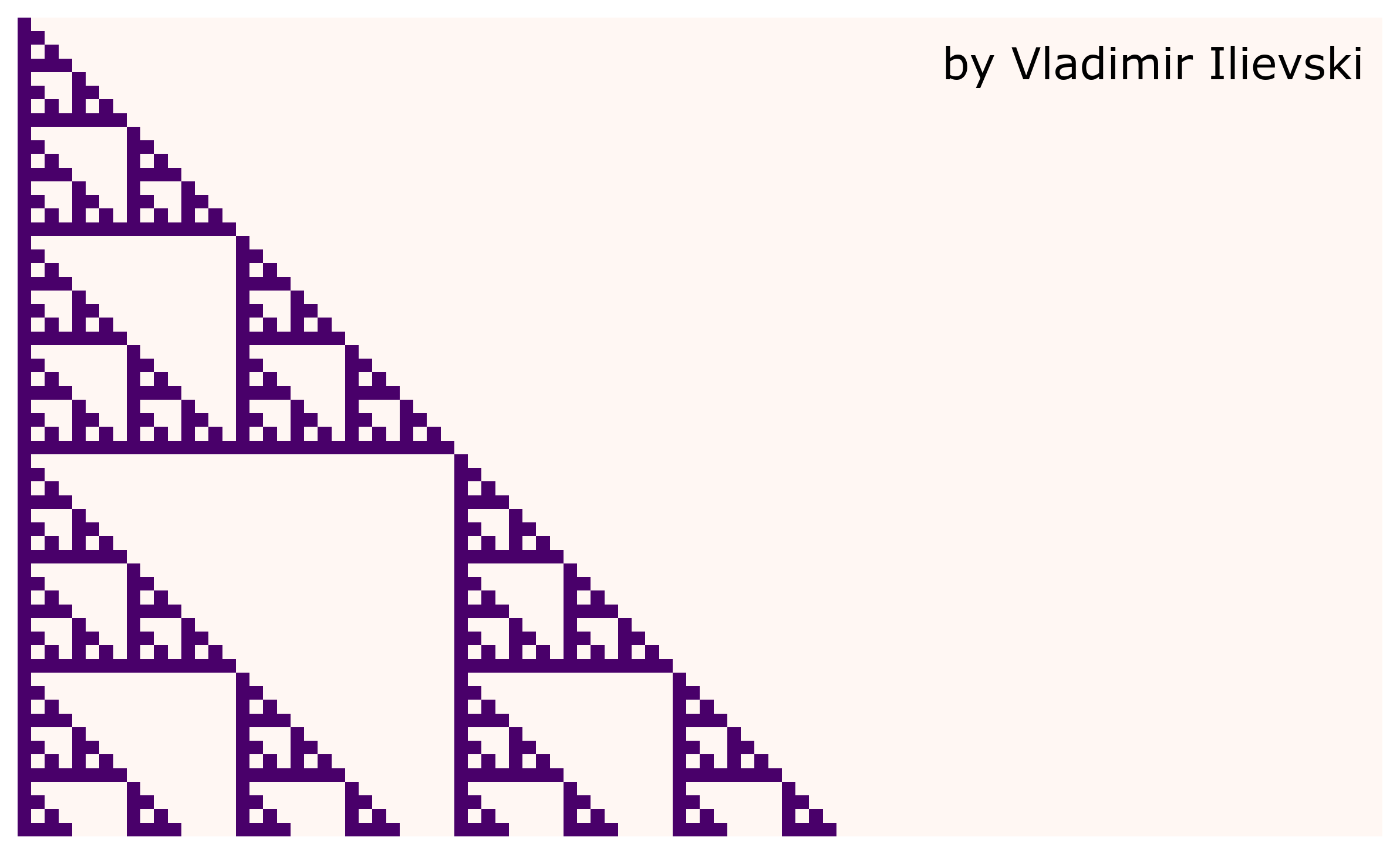
Fig. 6: Evolution of an elementary cellular automaton

Animated Visualization

Let’s put one cellular automaton in action and see how it looks like when it evolves in time. In order to do this, we use the Matplotlib Animation API to create an animation of the evolution process. We will use rule number 90 starting with one active cell at the center of the row.

If we set a sliding window over which we will observe the evolution over time of the cellular automaton, we get the following animation:

Fig. 7: Animation of the evolution of an elementary cellular automaton

The entire source code for the implementation of the elementary cellular automata can be found on GitHub.

If this is something you like and would like to receive similar posts, please subscribe to the mailing list below. For more information, please follow me on LinkedIn or Twitter.

Summary: Elementary but not simple

It is interesting to see the repeating pattern of triangles over the evolution of the cellular automaton above. However, this is not always the case. For example, it is proven that by using rule number 110 we can get a Turing-complete machine that is capable of universal computing which is pretty stunning for such a simple system.

To conclude, the elementary cellular automata and in general the cellular automata are very interesting phenomenon in the world of computing. With a simple set of rules motivated by the evolution of the living organisms, it is possible to construct universal machines capable of computing everything.

References

[1] Stephen Wolfram, "A New Kind of Science" (2002), Wolfram Media